Models

The following models are currently implemented in OpenCMP. In general, all models are expected to include a standard Galerkin finite element method formulation, a discontinuous Galerkin formulation, and a diffuse interface formulation. Nonlinear models are further expected to include formulations for Oseen-style linearization and IMEX linearization. The following sections provide the weak forms for all implemented formulations of the available models.

Poisson Equation

The Poisson equation takes the following form on a simulation domain $\Omega$ . There are three possible types of boundary condition - Dirichlet, Neumann, and Robin - applied on boundary regions $\Gamma_D$ , $\Gamma_N$ , and $\Gamma_R$ respectively.

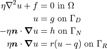
$\eta \nabla^2 u + f &= 0 \mbox{ in } \Omega \\ u &= g \mbox{ on } \Gamma_D \\ -\eta \bm{n} \cdot \bm{\nabla} u &= h \mbox{ on } \Gamma_N \\ \eta \bm{n} \cdot \bm{\nabla} u &= r(u - q) \mbox{ on } \Gamma_R$

where $\eta$ is a constant typically taken to be the diffusivity and $f$ is some source function.

The different formulations of the Poisson equation finite element weak form are given below. Note that in all cases $v$ is the trial function. In the case of the discontinuous Galerkin method, $\{\}$ and $[[]]$ refer to the average and jump operators respectively and $\alpha$ is the penalty coefficient. In the case of the diffuse interface method, $\phi$ is the phase field, $\{ \phi_{const} \}$ are masks for different boundary condition regions, and $\beta$ is the Nitsche method penalty parameter. Also note that for the diffuse interface method all integrals become volume integrals over the enclosing simple domain $\kappa$ .

Standard Galerkin Finite Element Formulation

The standard Galerkin finite element method formulation is as follows:

$\int_{\Omega} \bm{\nabla} u \cdot \bm{\nabla} v \: dx + \int_{\Gamma_N} \frac{1}{\eta} hv \: ds - \int_{\Gamma_R} \frac{1}{\eta} vr \left( u - q \right) \: ds = \int_{\Omega} \frac{1}{\eta} fv \: dx$

Dirichlet boundary conditions are imposed strongly by setting values at applicable boundary degrees of freedom.

Discontinuous Galerkin Formulation

The discontinuous Galerkin formulation is as follows:

$&\sum_{\mathcal{K} \in \mathcal{T}} \int_{\mathcal{K}} \bm{\nabla} u \cdot \bm{\nabla} v \: dx \\ - &\sum_{\mathcal{F} \in \mathcal{F}_I} \int_{\mathcal{F}} \left( [[u\bm{n}]] \cdot \{ \bm{\nabla} v \} + [[v\bm{n}]] \cdot \{ \bm{\nabla} u \} - \alpha [[u]] [[v]] \right) \: ds \\ - &\sum_{\mathcal{F} \in \mathcal{F}_D} \int_{\mathcal{F}} \left( \bm{n} \cdot \left( u - g \right) \bm{\nabla} v + \bm{n} \cdot v \bm{\nabla} u - \alpha \left( u - g \right) v \right) \: ds \\ - &\sum_{\mathcal{F} \in \mathcal{F}_N} \int_{\mathcal{F}} \frac{1}{\eta} vh \: ds + \sum_{\mathcal{F} \in \mathcal{F}_R} \int_{\mathcal{F}} \frac{1}{\eta} vr\left( u - q \right) \: ds \\ = &\sum_{\mathcal{K} \in \mathcal{T}} \int_{\mathcal{K}} \frac{1}{\eta} fv \: dx$

where volume integrals are over individual mesh elements $\mathcal{K}$ then summed over the entire triangulation $\mathcal{T}$ . Surface integrals are over mesh element facets $\mathcal{F}$ and summed over either interior facets $\mathcal{F}_I$ or boundary facets $\mathcal{F}_D$ , $\mathcal{F}_N$ , and $\mathcal{F}_R$ .

Diffuse Interface Formulation

The diffuse interface formulation is as follows for the standard Galerkin finite element method:

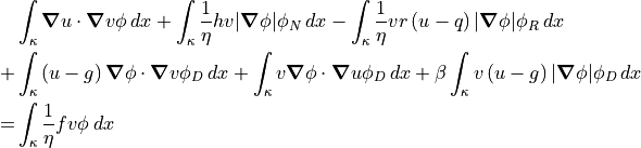
$&\int_{\kappa} \bm{\nabla} u \cdot \bm{\nabla} v \phi \: dx + \int_{\kappa} \frac{1}{\eta} hv \lvert \bm{\nabla} \phi \rvert \phi_N \: dx - \int_{\kappa} \frac{1}{\eta} vr \left( u - q \right) \lvert \bm{\nabla} \phi \rvert \phi_R \: dx \\ + &\int_{\kappa} \left( u - g \right) \bm{\nabla} \phi \cdot \bm{\nabla} v \phi_D \: dx + \int_{\kappa} v \bm{\nabla} \phi \cdot \bm{\nabla} u \phi_D \: dx + \beta \int_{\kappa} v \left( u - g \right) \lvert \bm{\nabla} \phi \rvert \phi_D \: dx \\ = &\int_{\kappa} \frac{1}{\eta} fv \phi \: dx$

and for the discontinuous Galerkin method:

$&\sum_{\mathcal{K} \in \mathcal{T}} \int_{\mathcal{K}} \bm{\nabla} u \cdot \bm{\nabla} v \phi \: dx \\ - &\sum_{\mathcal{F} \in \mathcal{F}_I} \int_{\mathcal{F}} \left( [[u\bm{n}]] \cdot \{ \bm{\nabla} v \} + [[v\bm{n}]] \cdot \{ \bm{\nabla} u \} - \alpha [[u]] [[v]] \right) \phi \: ds \\ + &\sum_{\mathcal{K} \in \mathcal{T}} \int_{\mathcal{K}} \left( \left( u - g \right) \bm{\nabla} \phi \cdot \bm{\nabla} v + v \bm{\nabla} \phi \cdot \bm{\nabla} u + \beta \left( u - g \right) v \lvert \bm{\nabla} \phi \rvert \right) \phi_D \: dx \\ + &\sum_{\mathcal{K} \in \mathcal{T}} \int_{\mathcal{K}} \frac{1}{\eta} vh \lvert \bm{\nabla} \phi \rvert \phi_N \: dx + \sum_{\mathcal{K} \in \mathcal{T}} \int_{\mathcal{K}} \frac{1}{\eta} vr\left( u - q \right) \lvert \bm{\nabla} \phi \rvert \phi_R \: dx \\ = &\sum_{\mathcal{K} \in \mathcal{T}} \int_{\mathcal{K}} \frac{1}{\eta} fv \phi \: dx$

Stokes Equations

The Stokes equations take the following form on a simulation domain $\Omega$ . There are two possible types of boundary condition - velocity Dirichlet and normal stress - applied on boundary regions $\Gamma_D$ and $\Gamma_S$ respectively.

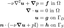
$-\nu \nabla^2 \bm{u} + \bm{\nabla} p &= \bm{f} \mbox{ in } \Omega \\ \bm{\nabla} \cdot \bm{u} &= 0 \mbox{ in } \Omega \\ \bm{u} &= \bm{g} \mbox{ on } \Gamma_D \\ \bm{n} \cdot \left(-\nu \bm{\nabla} \bm{u} + p \mathbb{I} \right) &= \bm{h} \mbox{ on } \Gamma_S$

where $\bm{u}$ is the velocity and $p$ is the pressure. Furthermore, $\nu$ is the constant kinematic viscosity and $f$ is some body force.

The different formulations of the Stokes equations finite element weak form are given below. Note that in all cases $\bm{v}$ and $q$ are the trial functions for velocity and pressure respectively. In the case of the discontinuous Galerkin method, $\{\}$ and $[[]]$ refer to the average and jump operators respectively and $\alpha$ is the penalty coefficient. In the case of the diffuse interface method, $\phi$ is the phase field, $\{ \phi_{const} \}$ are masks for different boundary condition regions, and $\beta$ is the Nitsche method penalty parameter. Also note that for the diffuse interface method all integrals become volume integrals over the enclosing simple domain $\kappa$ .

Standard Galerkin Finite Element Formulation

The standard Galerkin finite element method formulation is as follows:

$\int_{\Omega} \left( \nu \bm{\nabla} \bm{u} : \bm{\nabla} \bm{v} - p \left( \bm{\nabla} \cdot \bm{v} \right) - q \left( \bm{\nabla} \cdot \bm{u} \right) \right) \: dx + \int_{\Gamma_S} \bm{v} \cdot \bm{h} \: ds &= \int_{\Omega} \bm{v} \cdot \bm{f} \: dx$

Dirichlet boundary conditions are imposed strongly by setting values at applicable boundary degrees of freedom.

Discontinuous Galerkin Formulation

The discontinuous Galerkin formulation is as follows:

$&\sum_{\mathcal{K} \in \mathcal{T}} \int_{\mathcal{K}} \left( \nu \bm{\nabla} \bm{u} : \bm{\nabla} \bm{v} - p \left( \bm{\nabla} \cdot \bm{v} \right) - q \left( \bm{\nabla} \cdot \bm{u} \right) \right) \: dx \\ - &\sum_{\mathcal{F} \in \mathcal{F}_I} \int_{\mathcal{F}} \nu \left( [[\bm{u}\bm{n}]] : \{ \bm{\nabla} \bm{v} \} + [[\bm{v}\bm{n}]] : \{ \bm{\nabla} \bm{u} \} - \alpha [[\bm{u} \bm{n}]] : [[\bm{v} \bm{n}]] \right) \: ds \\ - &\sum_{\mathcal{F} \in \mathcal{F}_D} \int_{\mathcal{F}} \nu \left( \left( \bm{u} - \bm{g} \right) \bm{n} : \bm{\nabla} \bm{v} + \bm{v} \bm{n} : \bm{\nabla} \bm{u} - \alpha \left( \bm{u} - \bm{g} \right) \cdot \bm{v} \right) \: ds \\ - &\sum_{\mathcal{F} \in \mathcal{F}_S} \int_{\mathcal{F}} \bm{v} \cdot \bm{h} \: ds \\ = &\sum_{\mathcal{K} \in \mathcal{T}} \int_{\mathcal{K}} \bm{v} \cdot \bm{f} \: dx$

where volume integrals are over individual mesh elements $\mathcal{K}$ then summed over the entire triangulation $\mathcal{T}$ . Surface integrals are over mesh element facets $\mathcal{F}$ and summed over either interior facets $\mathcal{F}_I$ or boundary facets $\mathcal{F}_D$ and $\mathcal{F}_S$ .

Diffuse Interface Formulation

The diffuse interface formulation is as follows for the standard Galerkin finite element method:

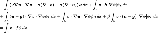
$&\int_{\kappa} \left( \nu \bm{\nabla} \bm{u} : \bm{\nabla} \bm{v} - p \left( \bm{\nabla} \cdot \bm{v} \right) - q \left( \bm{\nabla} \cdot \bm{u} \right) \right) \phi \: dx + \int_{\kappa} \bm{v} \cdot \bm{h} \lvert \bm{\nabla} \phi \rvert \phi_S \: dx \\ + &\int_{\kappa} \left( \bm{u} - \bm{g} \right) \cdot \bm{\nabla} \bm{v} \cdot \bm{\nabla} \phi \phi_D \: dx + \int_{\kappa} \bm{v} \cdot \bm{\nabla} \bm{u} \cdot \bm{\nabla} \phi \phi_D \: dx + \beta \int_{\kappa} \bm{v} \cdot \left( \bm{u} - \bm{g} \right) \lvert \bm{\nabla} \phi \rvert \phi_D \: dx \\ = &\int_{\kappa} \bm{v} \cdot \bm{f} \phi \: dx$

and for the discontinuous Galerkin method:

$&\sum_{\mathcal{K} \in \mathcal{T}} \int_{\mathcal{K}} \left( \nu \bm{\nabla} \bm{u} : \bm{\nabla} \bm{v} - p \left( \bm{\nabla} \cdot \bm{v} \right) - q \left( \bm{\nabla} \cdot \bm{u} \right) \right) \phi \: dx \\ - &\sum_{\mathcal{F} \in \mathcal{F}_I} \int_{\mathcal{F}} \nu \left( [[\bm{u}\bm{n}]] : \{ \bm{\nabla} \bm{v} \} + [[\bm{v}\bm{n}]] : \{ \bm{\nabla} \bm{u} \} - \alpha [[\bm{u} \bm{n}]] : [[\bm{v} \bm{n}]] \right) \phi \: ds \\ + &\sum_{\mathcal{K} \in \mathcal{T}} \int_{\mathcal{K}} \nu \left( \left( \bm{u} - \bm{g} \right) \bm{\nabla} \phi : \bm{\nabla} \bm{v} + \bm{v} \bm{\nabla} \phi : \bm{\nabla} \bm{u} - \beta \left( \bm{u} - \bm{g} \right) \cdot \bm{v} \lvert \bm{\nabla} \phi \rvert \right) \phi_D \: dx \\ - &\sum_{\mathcal{K} \in \mathcal{T}} \int_{\mathcal{K}} \bm{v} \cdot \bm{h} \lvert \bm{\nabla} \phi \rvert \phi_S \: dx \\ = &\sum_{\mathcal{K} \in \mathcal{T}} \int_{\mathcal{K}} \bm{v} \cdot \bm{f} \phi \: dx$

Incompressible Navier-Stokes Equations

The incompressible Navier-Stokes equations take the following form on a simulation domain $\Omega$ . There are two possible types of boundary condition - velocity Dirichlet and normal stress - applied on boundary regions $\Gamma_D$ and $\Gamma_S$ respectively.

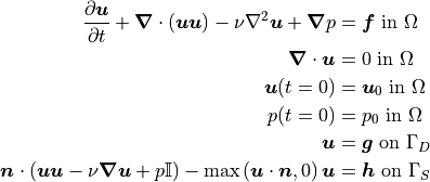
$\frac{\partial \bm{u}}{\partial t} + \bm{\nabla} \cdot \left( \bm{u} \bm{u} \right) - \nu \nabla^2 \bm{u} + \bm{\nabla} p &= \bm{f} \mbox{ in } \Omega \\ \bm{\nabla} \cdot \bm{u} &= 0 \mbox{ in } \Omega \\ \bm{u}(t=0) &= \bm{u}_0 \mbox{ in } \Omega \\ p(t=0) &= p_0 \mbox{ in } \Omega \\ \bm{u} &= \bm{g} \mbox{ on } \Gamma_D \\ \bm{n} \cdot \left(\bm{u} \bm{u} - \nu \bm{\nabla} \bm{u} + p \mathbb{I} \right) - \max \left( \bm{u} \cdot \bm{n},0 \right) \bm{u} &= \bm{h} \mbox{ on } \Gamma_S$

where $\bm{u}$ is the velocity and $p$ is the pressure. Furthermore, $\nu$ is the constant kinematic viscosity and $f$ is some body force. When Oseen-style linearization is used to linearize the nonlinear convection term, one velocity in said term with be replaced by a known velocity field $\bm{w}$ (usually the velocity from the previous time step).

The different formulations of the incompressible Navier-Stokes equations finite element weak form are given below. Note that in all cases $\bm{v}$ and $q$ are the trial functions for velocity and pressure respectively. In the case of the discontinuous Galerkin method, $\{\}$ and $[[]]$ refer to the average and jump operators respectively and $\alpha$ is the penalty coefficient. In the case of the diffuse interface method, $\phi$ is the phase field, $\{ \phi_{const} \}$ are masks for different boundary condition regions, and $\beta$ is the Nitsche method penalty parameter. Also note that for the diffuse interface method all integrals become volume integrals over the enclosing simple domain $\kappa$ .

Standard Galerkin Finite Element Formulation

The standard Galerkin finite element method formulation is as follows for Oseen-style linearization:

$&\int_{\Omega} \left( \bm{v} \cdot \frac{\partial \bm{u}}{\partial t} - \bm{u} \bm{w} : \bm{\nabla} \bm{v} + \nu \bm{\nabla} \bm{u} : \bm{\nabla} \bm{v} - p \left( \bm{\nabla} \cdot \bm{v} \right) - q \left( \bm{\nabla} \cdot \bm{u} \right) \right) \: dx \\ + &\int_{\Gamma_S} \bm{v} \cdot \left( \bm{h} + \max \left( \bm{w} \cdot \bm{n}, 0 \right) \bm{u} \right) \: ds \\ = &\int_{\Omega} \bm{v} \cdot \bm{f} \: dx$

and IMEX time discretization:

$&\int_{\Omega} \left( \bm{v} \cdot \frac{\partial \bm{u}}{\partial t} + \nu \bm{\nabla} \bm{u} : \bm{\nabla} \bm{v} - p \left( \bm{\nabla} \cdot \bm{v} \right) - q \left( \bm{\nabla} \cdot \bm{u} \right) \right) \: dx \\ + &\int_{\Gamma_S} \bm{v} \cdot \left( \bm{h} + \max \left( \bm{w} \cdot \bm{n},0 \right) \bm{u} \right) \: ds \\ = &\int_{\Omega} \left( \bm{v} \cdot \bm{f} - \bm{u} \cdot \bm{\nabla} \bm{u} \cdot \bm{v} \right) \: dx$

In both cases, Dirichlet boundary conditions are imposed strongly by setting values at applicable boundary degrees of freedom.

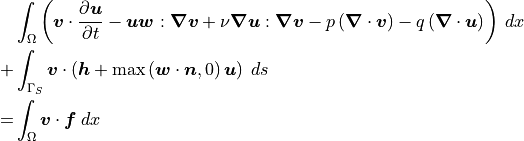
Discontinuous Galerkin Formulation

The discontinuous Galerkin formulation is as follows for Oseen-style linearization:

$&\sum_{\mathcal{K} \in \mathcal{T}} \int_{\mathcal{K}} \left( \bm{v} \cdot \frac{\partial \bm{u}}{\partial t} - \bm{u} \bm{w} : \bm{\nabla} \bm{v} + \nu \bm{\nabla} \bm{u} : \bm{\nabla} \bm{v} - p \left( \bm{\nabla} \cdot \bm{v} \right) - q \left( \bm{\nabla} \cdot \bm{u} \right) \right) \: dx \\ + &\sum_{\mathcal{F} \in \mathcal{F}_I} \int_{\mathcal{F}} [[\bm{v} \bm{n}]] : \left( \{ \bm{u} \} \left( \bm{w} \cdot \bm{n} \right) \bm{n} + \frac{1}{2} \left( \bm{u}^+ - \bm{u}^- \right) \lvert \bm{w} \cdot \bm{n} \rvert \bm{n} \right) \: ds \\ - &\sum_{\mathcal{F} \in \mathcal{F}_I} \int_{\mathcal{F}} \nu \left( [[\bm{u}\bm{n}]] : \{ \bm{\nabla} \bm{v} \} + [[\bm{v}\bm{n}]] : \{ \bm{\nabla} \bm{u} \} - \alpha [[\bm{u} \bm{n}]] : [[\bm{v} \bm{n}]] \right) \: ds \\ + &\sum_{\mathcal{F} \in \mathcal{F}_D} \int_{\mathcal{F}} \bm{v} \bm{n} : \left( \frac{1}{2} \left( \bm{u} + \bm{g} \right) \left( \bm{w} \cdot \bm{n} \right) \bm{n} + \frac{1}{2} \left( \bm{u} - \bm{g} \right) \lvert \bm{w} \cdot \bm{n} \rvert \bm{n} \right) \: ds \\ - &\sum_{\mathcal{F} \in \mathcal{F}_D} \int_{\mathcal{F}} \nu \left( \left( \bm{u} - \bm{g} \right) \bm{n} : \bm{\nabla} \bm{v} + \bm{v} \bm{n} : \bm{\nabla} \bm{u} - \alpha \left( \bm{u} - \bm{g} \right) \cdot \bm{v} \right) \: ds \\ + &\sum_{\mathcal{F} \in \mathcal{F}_S} \int_{\mathcal{F}} \bm{v} \cdot \left( \bm{h} + \max \left( \bm{w} \cdot \bm{n}, 0 \right) \bm{u} \right) \: ds \\ = &\sum_{\mathcal{K} \in \mathcal{T}} \int_{\mathcal{K}} \bm{v} \cdot \bm{f} \: dx$

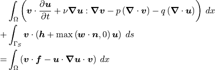
and IMEX time discretization:

$&\sum_{\mathcal{K} \in \mathcal{T}} \int_{\mathcal{K}} \left( \bm{v} \cdot \frac{\partial \bm{u}}{\partial t} + \nu \bm{\nabla} \bm{u} : \bm{\nabla} \bm{v} - p \left( \bm{\nabla} \cdot \bm{v} \right) - q \left( \bm{\nabla} \cdot \bm{u} \right) \right) \: dx \\ - &\sum_{\mathcal{F} \in \mathcal{F}_I} \int_{\mathcal{F}} \nu \left( [[\bm{u}\bm{n}]] : \{ \bm{\nabla} \bm{v} \} + [[\bm{v}\bm{n}]] : \{ \bm{\nabla} \bm{u} \} - \alpha [[\bm{u} \bm{n}]] : [[\bm{v} \bm{n}]] \right) \: ds \\ - &\sum_{\mathcal{F} \in \mathcal{F}_D} \int_{\mathcal{F}} \nu \left( \left( \bm{u} - \bm{g} \right) \bm{n} : \bm{\nabla} \bm{v} + \bm{v} \bm{n} : \bm{\nabla} \bm{u} - \alpha \left( \bm{u} - \bm{g} \right) \cdot \bm{v} \right) \: ds \\ + &\sum_{\mathcal{F} \in \mathcal{F}_S} \int_{\mathcal{F}} \bm{v} \cdot \left( \bm{h} + \max \left( \bm{w} \cdot \bm{n}, 0 \right) \bm{u} \right) \: ds \\ = &\sum_{\mathcal{K} \in \mathcal{T}} \int_{\mathcal{K}} \left( \bm{v} \cdot \bm{f} - \bm{u} \cdot \bm{\nabla} \bm{u} \cdot \bm{v} \right) \: dx$

In both cases, volume integrals are over individual mesh elements $\mathcal{K}$ then summed over the entire triangulation $\mathcal{T}$ . Surface integrals are over mesh element facets $\mathcal{F}$ and summed over either interior facets $\mathcal{F}_I$ or boundary facets $\mathcal{F}_D$ and $\mathcal{F}_S$ .

Diffuse Interface Formulation

The diffuse interface formulation is as follows for the standard Galerkin finite element method using Oseen-style linearization:

$&\int_{\kappa} \left( \bm{v} \cdot \frac{\partial \bm{u}}{\partial t} - \bm{u} \bm{w} : \bm{\nabla} \bm{v} + \nu \bm{\nabla} \bm{u} : \bm{\nabla} \bm{v} - p \left( \bm{\nabla} \cdot \bm{v} \right) - q \left( \bm{\nabla} \cdot \bm{u} \right) \right) \phi \: dx \\ + &\int_{\kappa} \bm{v} \cdot \left( \bm{h} + \max \left( \bm{w} \cdot \bm{n}, 0 \right) \bm{u} \right) \lvert \bm{\nabla} \phi \rvert \phi_S \: dx \\ + &\int_{\kappa} \left( \bm{u} - \bm{g} \right) \cdot \bm{\nabla} \bm{v} \cdot \bm{\nabla} \phi \phi_D \: dx + \int_{\kappa} \bm{v} \cdot \bm{\nabla} \bm{u} \cdot \bm{\nabla} \phi \phi_D \: dx + \beta \int_{\kappa} \bm{v} \cdot \left( \bm{u} - \bm{g} \right) \lvert \bm{\nabla} \phi \rvert \phi_D \: dx \\ = &\int_{\Omega} \bm{v} \cdot \bm{f} \: dx$

and IMEX time discretization:

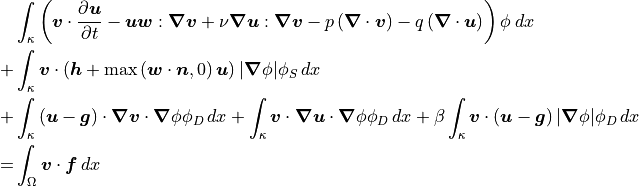
$&\int_{\kappa} \left( \bm{v} \cdot \frac{\partial \bm{u}}{\partial t} + \nu \bm{\nabla} \bm{u} : \bm{\nabla} \bm{v} - p \left( \bm{\nabla} \cdot \bm{v} \right) - q \left( \bm{\nabla} \cdot \bm{u} \right) \right) \phi \: dx \\ + &\int_{\kappa} \bm{v} \cdot \left( \bm{h} + \max \left( \bm{w} \cdot \bm{n},0 \right) \bm{u} \right) \lvert \bm{\nabla} \phi \rvert \phi_S \: dx \\ + &\int_{\kappa} \left( \bm{u} - \bm{g} \right) \cdot \bm{\nabla} \bm{v} \cdot \bm{\nabla} \phi \phi_D \: dx + \int_{\kappa} \bm{v} \cdot \bm{\nabla} \bm{u} \cdot \bm{\nabla} \phi \phi_D \: dx + \beta \int_{\kappa} \bm{v} \cdot \left( \bm{u} - \bm{g} \right) \lvert \bm{\nabla} \phi \rvert \phi_D \: dx \\ = &\int_{\kappa} \left( \bm{v} \cdot \bm{f} - \bm{u} \cdot \bm{\nabla} \bm{u} \cdot \bm{v} \right) \phi \: dx$

The diffuse interface formulation is as follows for the discontinuous Galerkin method using Oseen-style linearization:

$&\sum_{\mathcal{K} \in \mathcal{T}} \int_{\mathcal{K}} \left( \bm{v} \cdot \frac{\partial \bm{u}}{\partial t} - \bm{u} \bm{w} : \bm{\nabla} \bm{v} + \nu \bm{\nabla} \bm{u} : \bm{\nabla} \bm{v} - p \left( \bm{\nabla} \cdot \bm{v} \right) - q \left( \bm{\nabla} \cdot \bm{u} \right) \right) \phi \: dx \\ + &\sum_{\mathcal{F} \in \mathcal{F}_I} \int_{\mathcal{F}} [[\bm{v} \bm{n}]] : \left( \{ \bm{u} \} \left( \bm{w} \cdot \bm{n} \right) \bm{n} + \frac{1}{2} \left( \bm{u}^+ - \bm{u}^- \right) \lvert \bm{w} \cdot \bm{n} \rvert \bm{n} \right) \: ds \\ - &\sum_{\mathcal{F} \in \mathcal{F}_I} \int_{\mathcal{F}} \nu \left( [[\bm{u}\bm{n}]] : \{ \bm{\nabla} \bm{v} \} + [[\bm{v}\bm{n}]] : \{ \bm{\nabla} \bm{u} \} - \alpha [[\bm{u} \bm{n}]] : [[\bm{v} \bm{n}]] \right) \: ds \\ - &\sum_{\mathcal{K} \in \mathcal{T}} \int_{\mathcal{K}} \bm{v} \cdot \left( \frac{1}{2} \left( \bm{u} + \bm{g} \right) \left( \bm{w} \cdot \bm{\nabla} \phi \right) + \frac{1}{2} \left( \bm{u} - \bm{g} \right) \lvert \bm{w} \cdot \bm{\nabla} \phi \rvert \right) \phi_D \: dx \\ + &\sum_{\mathcal{K} \in \mathcal{T}} \int_{\mathcal{K}} \nu \left( \left( \bm{u} - \bm{g} \right) \bm{\nabla} \phi : \bm{\nabla} \bm{v} + \bm{v} \bm{\nabla} \phi : \bm{\nabla} \bm{u} - \alpha \left( \bm{u} - \bm{g} \right) \cdot \bm{v} \lvert \bm{\nabla} \phi \rvert \right) \phi_D \: dx \\ + &\sum_{\mathcal{K} \in \mathcal{T}} \int_{\mathcal{K}} \bm{v} \cdot \left( \bm{h} + \max \left( \bm{w} \cdot \bm{n}, 0 \right) \bm{u} \right) \lvert \bm{\nabla} \phi \rvert \phi_D \: dx \\ = &\sum_{\mathcal{K} \in \mathcal{T}} \int_{\mathcal{K}} \bm{v} \cdot \bm{f} \phi \: dx$

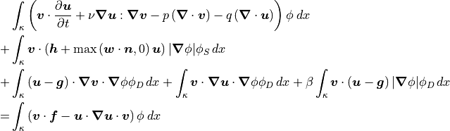
and IMEX time discretization:

$&\sum_{\mathcal{K} \in \mathcal{T}} \int_{\mathcal{K}} \left( \bm{v} \cdot \frac{\partial \bm{u}}{\partial t} + \nu \bm{\nabla} \bm{u} : \bm{\nabla} \bm{v} - p \left( \bm{\nabla} \cdot \bm{v} \right) - q \left( \bm{\nabla} \cdot \bm{u} \right) \right) \phi \: dx \\ - &\sum_{\mathcal{F} \in \mathcal{F}_I} \int_{\mathcal{F}} \nu \left( [[\bm{u}\bm{n}]] : \{ \bm{\nabla} \bm{v} \} + [[\bm{v}\bm{n}]] : \{ \bm{\nabla} \bm{u} \} - \alpha [[\bm{u} \bm{n}]] : [[\bm{v} \bm{n}]] \right) \phi \: ds \\ + &\sum_{\mathcal{K} \in \mathcal{T}} \int_{\mathcal{K}} \nu \left( \left( \bm{u} - \bm{g} \right) \bm{\nabla} \phi : \bm{\nabla} \bm{v} + \bm{v} \bm{\nabla} \phi : \bm{\nabla} \bm{u} - \alpha \left( \bm{u} - \bm{g} \right) \cdot \bm{v} \lvert \bm{\nabla} \phi \rvert \right) \phi_D \: dx \\ + &\sum_{\mathcal{K} \in \mathcal{T}} \int_{\mathcal{K}} \bm{v} \cdot \left( \bm{h} + \max \left( \bm{w} \cdot \bm{n}, 0 \right) \bm{u} \right) \lvert \bm{\nabla} \phi \rvert \phi_S \: dx \\ = &\sum_{\mathcal{K} \in \mathcal{T}} \int_{\mathcal{K}} \left( \bm{v} \cdot \bm{f} - \bm{u} \cdot \bm{\nabla} \bm{u} \cdot \bm{v} \right) \phi \: dx$

Multi-Component Flow

Note

To be written once discontinuous Galerkin and diffuse interface formulations are available for the multi-component flow model.