Warning

This example requires at least 16gb of RAM and could take several minutes to solve, depending on the number of threads specified and the performance of your CPU.

Tutorial 10 - Solving the Incompressible Navier-Stokes Equations (3D)

The files for this tutorial can be found in “examples/tutorial_10”.

Governing Equations

This tutorial will demonstrate how to solve the incompressible Navier-Stokes equations with Dirichlet and stress boundary conditions, as in Tutorial 6 - Solving the Incompressible Navier-Stokes Equations (2D), but now using geometry and conditions from a standard benchmark for 3D flow around a cylinder under conditions in which vortex shedding is not observed and a steady solution may be obtained (Re=20). The domain geometry is shown below:

Schematic of 3D immersed cylinder geometry.

There are no-slip conditions on all four channel walls and on the wall of the cylinder. The inlet velocity profile is parabolic,

$U(0, y, z) = [0, 0, 32 U_m x y (H - x) (H - y)/H^4]$

where Um = 0.45 m/s and H=0.41. Note that this deviates from the benchmark paper expression which has a factor of 16 instead of 32, which is a typographical error. There is a “do-nothing” outlet stress boundary condition and the kinematic viscosity of the liquid is 0.001.

Since the problem is assumed to have a steady-state, no initial conditions are required. However, to facilitate convergence of the steady solve the solution of the steady-state Stokes equations for the problem are used as the initial value for nonlinear iteration.

Additionally, this example will use OpenCMP’s built-in metric functionality, to compute the force vector on the immersed cylinder through integration of the surface traction over its boundary. Given that superficial velocity direction is the z-direction and the y-component is orthogonal to the flow direction, the corresponding force vector components are the drag and lift forces, respectively.

The Main Configuration Files

There are now two main configuration files: “config_IC” to specify the Stokes solve and “config” to specify the main incompressible Navier-Stokes solve.

“config_IC” is very similar to the main configuration file from Tutorial 6 - Solving the Incompressible Navier-Stokes Equations (2D) except for a few significant changes. First, since this is a low Reynolds number problem we may use a continuous Galerkin FEM, with standard Taylor-Hood elements:

[FINITE ELEMENT SPACE]
elements = u -> VectorH1
           p -> H1
interpolant_order = 2

Second, the linear solver and preconditioner are changed, along with the maximum number of nonlinear iterations, so that less memory will be used compared to a direct linear solver:

[SOLVER]
solver = CG
preconditioner = default
linearization_method = Oseen
nonlinear_tolerance = relative -> 1e-6
                      absolute -> 1e-6
nonlinear_max_iterations = 500

Third, the transient solve is disabled:

[TRANSIENT]
transient = False

The Boundary Condition Configuration File

The same boundary conditions are used for the Stokes solve and the incompressible Navier-Stokes solve so one boundary condition configuration file can be shared.

[DIRICHLET]
u = wall  -> [0.0, 0.0, 0.0]
    cyl  -> [0.0, 0.0, 0.0]
    inlet -> [0.0, 0.0, 32.0*0.45*x*y*(0.41-x)*(0.41-y)/0.41^4]

[STRESS]
stress = outlet -> [0.0, 0.0, 0.0]

Note that the wall of the cylinder has been marked “cyl” on the mesh.

The Initial Condition Configuration File

The Stokes solve is a steady-state solve so needs no initial conditions.

[STOKES]
all = all -> None

The incompressible Navier-Stokes solve does require initial conditions, but to facilitate convergence of the nonlinear solver the results of the Stokes solve will be saved to file and this file will be reloaded to provide initial conditions for the incompressible Navier-Stokes solve:

[INS]
all = all -> output/sol/stokes_0.0.sol

The Model Configuration File

The same model parameters are used for both solves.

[PARAMETERS]
kinematic_viscosity = all -> 0.001

[FUNCTIONS]
source = all -> [0.0, 0.0]

The Error Analysis Subdirectory

In this case, the exact solution is not known, but we do want to calculate the drag and lift coefficients from the simulation results in order to compare to the benchmark solutions which are included in the analysis metrics options that are (optionally) calculated by OpenCMP. These calculations are enabled by adding the metric “surface_traction”,

[METRICS] surface_traction = cyl

and indicating which surface it should be calculated on. In order to enable this calculation, we must add the following lines to the main configuration file (“config”),

[ERROR ANALYSIS] check_error = True

Running the Simulation

The simulation can be run from the command line; within the directory “examples/tutorial_10/:

Run the Stokes solve by calling python3 -m opencmp config_IC
Run the incompressible Navier-Stokes solve by calling python3 -m opencmp config.

The progress of a steady solution will be displayed in terms of number of nonlinear iterations and, within each nonlinear iteration, number of iterations of the linear solver. Once the simulation has finished the results can be visualized by opening “output/vtu/ins_0.0.vtu” in ParaView.

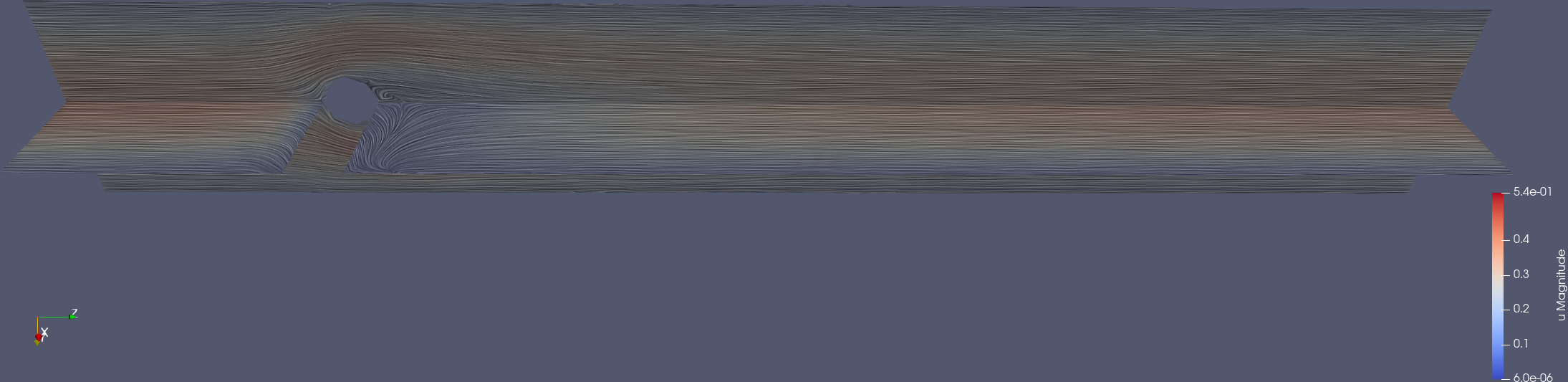
Visualization of steady solution velocity field using line integral convolutions on two different cross-sections.

The calculated force vector will be displayed following completion of the solve, the drag and lift coefficients may calculated based on the mean velocity,

$\bar{U} = \frac{4}{9} U_m$

and the following relations,

$C_D = \frac{2 F_z}{\rho \bar{U}^2 A} = 6.886$

$C_L = -\frac{2 F_y}{\rho \bar{U}^2 A} = 3.424e-2$

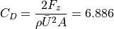
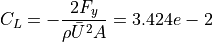
where the computed values for the coarse mesh used are 7.128 and 0.2054, respectively. Improved accuracy would result from mesh refinement and and recomputing, but this will significantly increase the memory and CPU requirements.