Tutorial 6 - Solving the Incompressible Navier-Stokes Equations (2D)

The files for this tutorial can be found in “examples/tutorial_6”.

Governing Equations

This tutorial will demonstrate how to solve the incompressible Navier-Stokes equations with Dirichlet and stress boundary conditions:

$\frac{\partial \bm{u}}{\partial t} + \bm{\nabla} \cdot \left( \bm{u} \bm{u} \right) - \nu \nabla^2 \bm{u} + \bm{\nabla} p &= \bm{f} \mbox{ in } \Omega \\ \bm{\nabla} \cdot \bm{u} &= 0 \mbox{ in } \Omega \\ \bm{u} &= \bm{g} \mbox{ on } \Gamma_D \\ \bm{n} \cdot \left(\bm{u} \bm{u} - \nu \bm{\nabla} \bm{u} + p \mathbb{I} \right) - \max (\bm{n} \cdot \bm{u}, 0) \bm{u} &= \bm{h} \mbox{ on } \Gamma_S$

These equations are nonlinear due to the convection term. The actual equations that will be solved are the Oseen equations, which linearize the incompressible Navier-Stokes equations by replacing one velocity with a wind ( $\bm{w}$ ):

$\frac{\partial \bm{u}}{\partial t} + \bm{\nabla} \cdot \left( \bm{u} \bm{w} \right) - \nu \nabla^2 \bm{u} + \bm{\nabla} p &= \bm{f} \mbox{ in } \Omega \\ \bm{\nabla} \cdot \bm{u} &= 0 \mbox{ in } \Omega \\ \bm{u} &= \bm{g} \mbox{ on } \Gamma_D \\ \bm{n} \cdot \left(\bm{u} \bm{w} - \nu \bm{\nabla} \bm{u} + p \mathbb{I} \right) - \max (\bm{n} \cdot \bm{w}, 0) \bm{u} &= \bm{h} \mbox{ on } \Gamma_S$

The specific example used in this tutorial is the Sch"{a}fer-Turek benchmark for 2D flow around a cylinder with vortex shedding. The domain geometry is shown below:

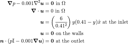
../_images/aafig-070ad3de272ee07d90eb297f60b9a3e9bc245d54.svg

There are no-slip conditions on both channel walls and on the wall of the cylinder. The inlet velocity profile is parabolic and there is a “do-nothing” outlet stress boundary condition. The kinematic viscosity is 0.001. The governing equations become as follows:

$\frac{\partial \bm{u}}{\partial t} + \bm{\nabla} \cdot \left( \bm{u} \bm{w} \right) - 0.001 \nabla^2 \bm{u} + \bm{\nabla} p &= \bm{0} \mbox{ in } \Omega \\ \bm{\nabla} \cdot \bm{u} &= 0 \mbox{ in } \Omega \\ \bm{u} &= \left( \frac{6}{0.41^2} \right) y (0.41 - y) \hat{x} \mbox{ at the inlet} \\ \bm{u} &= \bm{0} \mbox{ on the walls} \\ \bm{n} \cdot \left(\bm{u} \bm{w} - 0.001 \bm{\nabla} \bm{u} + p \mathbb{I} \right) - \max (\bm{n} \cdot \bm{w}, 0) \bm{u} &= \bm{0} \mbox{ at the outlet}$

Initial conditions must still be specified for the velocity and pressure. One way to ensure the initial conditions satisfy both the boundary conditions and the incompressibility constraint is to use the solution of the steady-state Stokes equations for the problem domain:

$\bm{\nabla} p - 0.001 \nabla^2 \bm{u} &= \bm{0} \mbox{ in } \Omega \\ \bm{\nabla} \cdot \bm{u} &= 0 \mbox{ in } \Omega \\ \bm{u} &= \left( \frac{6}{0.41^2} \right) y (0.41 - y) \hat{x} \mbox{ at the inlet} \\ \bm{u} &= \bm{0} \mbox{ on the walls} \\ \bm{n} \cdot \left( p \mathbb{I} - 0.001 \bm{\nabla} \bm{u} \right) &= \bm{0} \mbox{ at the outlet}$

The Main Configuration Files

There are now two main configuration files: “config_IC” to specify the Stokes solve and “config” to specify the main incompressible Navier-Stokes solve.

“config_IC” is very similar to the main configuration file from Tutorial 4 - Transient Solves. The only major change is the addition of a “curved_elements” parameter under the “[MESH]” heading. Since the cylinder in the interior of the simulation domain has curved walls, “curved_elements” is set to “True” to allow mesh element edges to follow the curvature of the cylinder up to the interpolant order.

[MESH]
filename = channel_w_cyl.vol
curved_elements = True

“config” also includes the “curved_elements” parameter. It is otherwise similar to the main configuration file from Tutorial 5 - Adaptive Time-Stepping. However, additional parameters are needed under the “[SOLVER]” heading to control the linearization.

The “linearization_method” parameter is only applicable to non-linear models and dictates whether the model will be linearized using the Oseen equations (or Oseen-type equations) or using an IMEX time discretization scheme. In this case, the Oseen equations are being used. The wind in the Oseen equations is obtained through Picard iterations using the previous time step’s velocity as an initial guess. Therefore, an error tolerance and maximum number of iterations must also be specified for the Picard iteration.

[SOLVER]
solver = default
preconditioner = default
linearization_method = Oseen
nonlinear_tolerance = relative -> 1e-6
                      absolute -> 1e-6
nonlinear_max_iterations = 3

Finally, the model type must be changed to “INS”.

[OTHER]
model = INS
run_dir = .
num_threads = 6

The Boundary Condition Configuration File

The same boundary conditions are used for the Stokes solve and the incompressible Navier-Stokes solve so one boundary condition configuration file can be shared.

[DIRICHLET]
u = wall  -> [0.0, 0.0]
inlet -> [6*y*(0.41-y)/(0.41*0.41), 0.0]
cyl   -> [0.0, 0.0]

[STRESS]
stress = outlet -> [0.0, 0.0]

Note that the wall of the cylinder has been marked “cyl” on the mesh.

The Initial Condition Configuration File

Different initial conditions are needed for each model, so they are given under separate headers in the initial condition configuration file.

The Stokes solve is a steady-state solve so needs no initial conditions.

[STOKES]
all = all -> None

The incompressible Navier-Stokes solve does require initial conditions. Unlike previous tutorials, the initial conditions are not known in closed-form. Instead, the results of the Stokes solve will be saved to file and this file will be reloaded to provide initial conditions for the incompressible Navier-Stokes solve. Data can only be loaded from .sol files and the given filepath points to where simulation results are saved. Alternatively, the results of the Stokes solve could be moved to a different folder and that filepath could be given.

[INS]
all = all -> output/sol/stokes_0.0.sol

The Model Configuration File

The same model parameters are used for both solves.

[PARAMETERS]
kinematic_viscosity = all -> 0.001

[FUNCTIONS]
source = all -> [0.0, 0.0]

The Error Analysis Subdirectory

In this case, the exact solution is not known, so the error analysis configuration file is left empty. Note that the divergence of the velocity and the velocity and pressure facet jumps could be calculated – they don’t require a reference solution – but aren’t.

Running the Simulation

The simulation can be run from the command line; within the directory “examples/tutorial_6/:

Run the Stokes solve by calling python3 -m opencmp config_IC
Run the incompressible Navier-Stokes solve by calling python3 -m opencmp config.

As usual, the progress of the transient simulation can be tracked from the print outs at each time step. Once the simulation has finished the results can be visualized by opening “output/transient.pvd” in ParaView.