Tutorial 2 - Convergence Testing

The files for this tutorial can be found in “examples/tutorial_2”.

Governing Equations

This tutorial will demonstrate OpenCMP’s various error analysis capabilities. The same problem will be used as in Tutorial 2 - Convergence Testing except with homogeneous Dirichlet boundary conditions:

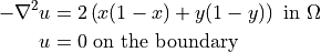
$-\nabla^2 u &= 2\left(x(1-x) + y(1-y)\right) \mbox{ in } \Omega \\ u &= 0 \mbox{ on the boundary}$

with the exact solution 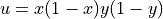$u = x(1-x)y(1-y)$ .

The Main Configuration File

Only a few changes need to be made to the main configuration file.

A different mesh will be used since only one boundary marker is necessary. Note that this mesh was constructed in Gmsh. For help generating Gmsh meshes that are compatible with OpenCMP see Using Gmsh with NGSolve.

[MESH]
filename = coarse_unit_square_1bc.msh

In this case the simulations results will not be saved to file.

[VISUALIZATION]
save_to_file = False

Instead a mesh convergence test will be conducted. OpenCMP gives options to compute various error metrics and to run convergence tests on mesh refinement or interpolant order refinement. This tutorial will check the convergence rate as the mesh is refined, so “h” is passed as the “convergence_test” value. The only model variable to test is “u”, but if the model had multiple variables each of their convergence rates could be checked. “num_refinements” sets the number of mesh refinements including the solve on the original mesh.

[ERROR ANALYSIS]
convergence_test = h -> u
num_refinements = 5

[OTHER]
model = Poisson
run_dir = .
num_threads = 2

The Boundary Condition Configuration File

The boundary condition configuration file must be modified to include only Dirichlet boundary conditions and the new mesh marker name.

[DIRICHLET]
u = bc -> 0.0

The Error Analysis Subdirectory

Information about what error metrics to compute during post-processing is held in the “config” file in the “ref_sol_dir” subdirectory.

First, the reference solutions to use when computing error metrics must be specified. In this tutorial this is the known exact solution and there is only one model variable for which to give a reference solution.

[REFERENCE SOLUTIONS]
u = x*(1-x)*y*(1-y)

The next section specifies which error metrics should be computed and for which model variables. In this case it is left blank since a convergence test is being run, which will compute the L2 norm between the simulation result and the reference solution.

Running the Simulation

The simulation can be run from the command line; within the directory examples/tutorial_2/ execute python3 -m opencmp config.

The usual warnings will print out about default values being used. Warnings will also print out about physical groups because a Gmsh mesh is being used. All of these can be ignored.

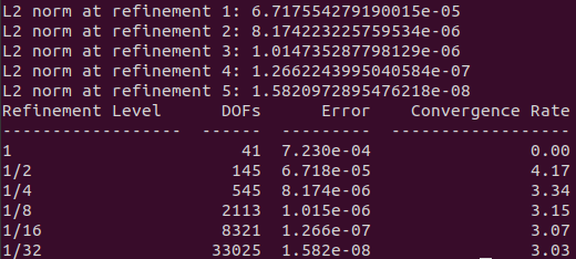
Of more interest are the results of the convergence test. The computed L2 norm will be printed out after each simulation at the various refinement levels. Then after the full test has finished a table will be printed out showing the convergence rates. This simulation used an interpolant order of 2 and superoptimal convergence rates (3+) should be seen.