Tutorial 9 - Diffuse Interface Method

The files for this tutorial can be found in “Examples/tutorial_9”.

Governing Equations

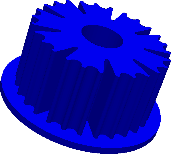
This tutorial will demonstrate how to use the diffuse interface method to approximate complex geometries with structured quadrilateral/hexahedral meshes.

The Main Configuration File

The main configuration file now includes and additional section to activate the diffuse interface method and point to the directory containing files specific to the diffuse interface method.

[DIM]
diffuse_interface_method = True
dim_dir = Examples/tutorial_9/dim_dir

The Diffuse Interface Method Configuration File

Within the diffuse interface method directory is the main configuration file for the diffuse interface method parameters - “dim_config”.

The first section of this configuration file governs the construction of the encompassing mesh and the diffuse interface. “mesh_dimension” is 3 since this is a 3-dimensional problem and “num_mesh_elements” controls the size of the mesh in each dimension. The spatial dimensions of the mesh come from “mesh_scale” and “mesh_offset” and should be slightly larger than the complex geometry being encompassed. In this case, the encompassing mesh extends from -2.5-2.5 in x and y and from -0.2-2.4 in z. Finally, “interface_width_parameter” controls the diffuseness of the diffuse interface approximation to the boundary of the complex geometry, with smaller values producing sharper interfaces for a given mesh element size.

[DIM]
mesh_dimension = 3
num_mesh_elements = x -> 80
                    y -> 80
                    z -> 80
mesh_scale = x -> 5
             y -> 5
             z -> 2.6
mesh_offset = x -> 2.5
              y -> 2.5
              z -> 0.2
interface_width_parameter = 0.01

The second section controls how boundary conditions are applied at the diffuse interface. In this case, there are two different boundary conditions applied on the bottom of the heat sink and its fans, so “multiple_bcs” is True. “remainder = True” means that once the region of the diffuse interface containing the bottom of the heat sink has been identified, the remainder of the diffuse interface with be assumed to correspond to the fan boundary condition, reducing computation time.

[DIM BOUNDARY CONDITIONS]
multiple_bcs = True
remainder = True

The third section contains additional information for the construction of the diffuse interface. “load_method” has three options, “generate”, “combine”, and “file” for the cases of (a) a diffuse interface that is constructed from an STL file of a complex geometry, (b) a diffuse interface that is constructed by combining multiple STL files at specified locations, and (c) a pregenerated diffuse interface that is loaded from a file. In this case, the diffuse interface will be generated on the spot from an STL file whose name must also be specified. Finally, the “save_to_file” option allows the diffuse interface and mesh to be saved to file after generation so they can later just be loaded.

[PHASE FIELDS]
load_method = generate
stl_filename = Examples/tutorial_9/dim_dir/led.stl
save_to_file = False

The Boundary Condition Configuration Files

The usual boundary condition file is empty, since boundary conditions are applied at the diffuse interface itself not at the boundaries of the encompassing mesh. Instead, boundary conditions are specified within the diffuse interface boundary condition configuration file “dim_dir/bc_dir/dim_bc_config”. There are the usual sections to specify Dirichlet, Neumann, or Robin boundary conditions. The two new sections, “VERTICES” and “CENTROIDS” are used to split the diffuse interface into different boundary condition regions.

[VERTICES]
bottom = Examples/tutorial_9/dim_dir/bc_dir/led_bottom.msh

[CENTROIDS]
bottom = <0.0, 0.0, 2.0>

[DIRICHLET]

[NEUMANN]
u = bottom -> Examples/tutorial_9/dim_dir/bc_dir/bottom_bc.sol

[ROBIN]
u = remainder -> 0.00124, 0.0

The Initial Condition Configuration File

No initial condition is needed for this steady-state problem.

[Poisson]
u = all -> None

The Model Configuration File

The model configuration file contains the usual model parameters and model functions for the Poisson equation

[PARAMETERS]
diffusion_coefficient = all -> 1.0

[FUNCTIONS]
source = all -> 0.0

The Error Analysis Subdirectory

In this case, the exact solution is not known, so the error analysis configuration file is left empty.

Running the Simulation

The simulation can be run from the command line; within the directory “examples/tutorial_9/”:

1. Execute python3 -m opencmp config, note that this is a computationally intensive simulation and num_threads is set to 4, but should be increased to your physical core count.

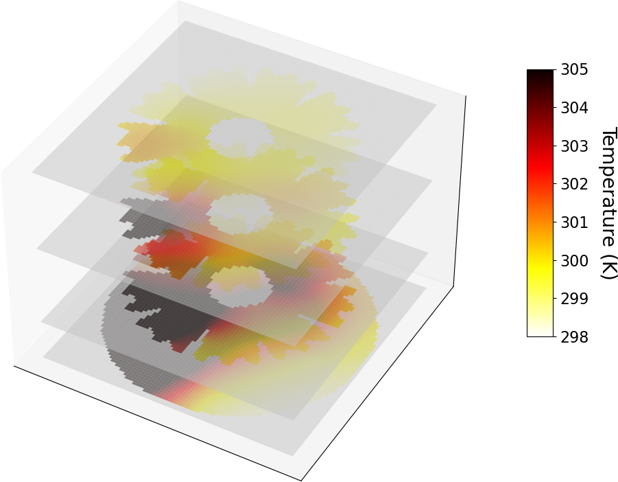
2. Execute python3 visualization to see a sample visualization (below).

Below is a cross section of the temperature field: